Dynamic labor supply

Setting the environment

The state space is given by age, producitivity and asset level. We consider the separable utility function over leisure and consumption. We fix all parameters. WE also consider a simple end of life value.

We prepare the wage realizations in each state and the value function.

p    = list(nx=30,na=40,nb=100,nh=10,gamma = 2, eta=-1.5 , lambda=0.1,r=0.02,beta=5,fc=1)
V    = array(0,c(p$na,p$nx,p$nb))
X    = exp(  qnorm((1:(p$nx))/(p$nx+1)))  
B    = c(0,exp(seq(log(min(X)),log(max(X/p$r)),l=p$nb-1)))
H    = seq(0,1,l=p$nh)
wage = X

# transition matrix on productivity
X1 = spread(X,1,p$nx);X2 = spread(X,2,p$nx);
Gx = dnorm(log(X2)-log(X1))
Gx = Gx/spread(rowSums(Gx),2,p$nx)
persp(Gx)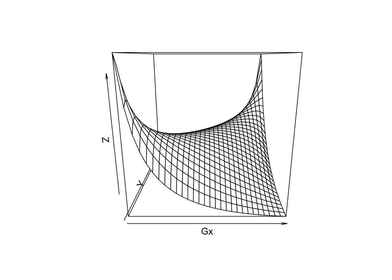

We then solve the dynamic problem recursively. In the last period, we let the agent choose a single consumption and hours value that will make asset level 0.

First step is to solve the final period problem. We assume that the agent has a access to a producitivity which is a thrid of the last period one, and then choose hours and consumption to make asset to 0.

t.final = tensorFunction(R[b,w,h] ~  ((W[w]*H[h] + r*B[b])^(1+eta))/(1+eta) - beta*((H[h])^(1+gamma))/(1+gamma) - I(H[h]>0)*fc)
VV      = t.final(X/3,H,B,p$r,p$eta,p$beta,p$gamma,p$fc)
Vf      = aaply(VV,c(1,2),max,na.rm=T)

# plotting the function
ggplot(melt(Vf,c("b","x")),aes(x=b,y=value,color=x,group=x))+geom_line() + theme_bw() + scale_x_continuous("asset position")

We then solve the values recursively

V[p$na,,] = t(Vf)/p$r

# prepare tensor that computes the Q value for each b,x,h,b2
t.cur = tensorFunction(R[b,x,h,b2] ~  ((W[x]*H[h] - B[b2] + (1+r)*B[b])^(1+eta))/(1+eta) - beta*((H[h])^(1+gamma))/(1+gamma) + rho*VV[x,b2] - I(H[h]>0)*fc )

B.pol = V*0
H.pol = V*0

for (age in (p$na-1):1) {
  # compute expected value tomorrow
  EV = Gx %*% V[age+1,,]
  # compute values at each control variables
  Vn = t.cur(W=X*exp(p$lambda * age/p$na) ,H,B,EV,p$r,p$eta,p$beta,p$gamma,1/(1+p$r),p$fc)
  # we need to choose the asset tomorrow and hours (which then gives consumption)
  V[age,,] = t(aaply(Vn,c(1,2),max,na.rm=T))
  # extract policy
  pol = aaply(Vn,c(1,2),function(A) which(A==max(A,na.rm=T),arr.ind = T,useNames = T))
  B.pol[age,,] = t(pol[,,2])
  H.pol[age,,] = t(pol[,,1])
  cat(".")
}

## .......................................

# let's plot hours at fix x and b over time
rr= data.table(melt(H.pol[,,25],c("age","x")))
ggplot(rr[x %in% c(5,10,15,20,25)][age<40],aes(x=age,y=value,color=x,group=x)) + geom_line()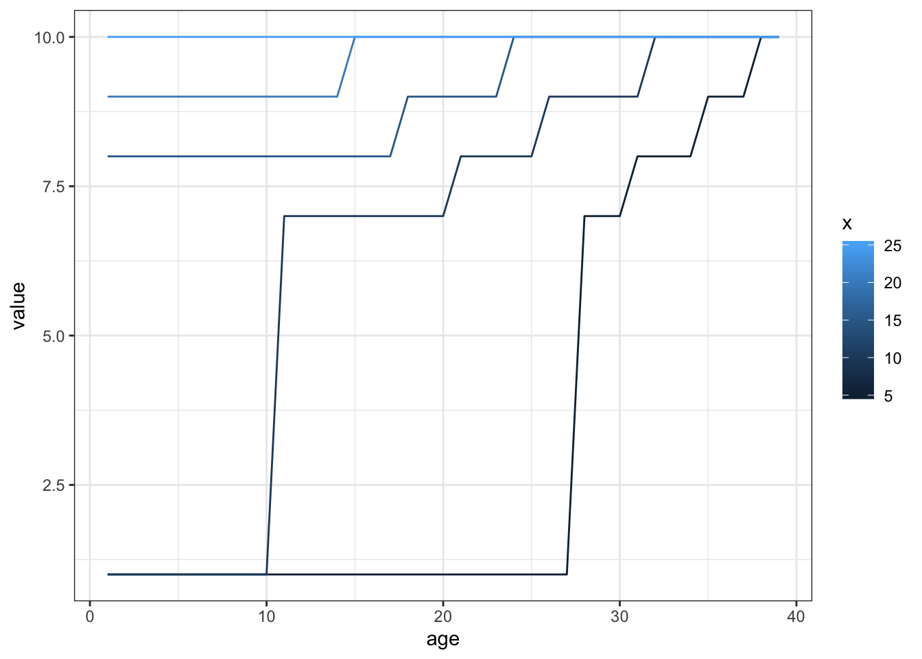

Simulating data

Finally we simulate some data

simdata = data.frame()
D = array(0,c(p$na-1,6))
colnames(D) = c("i","x","b","h","b2","age")
  
for (i in 1:1000) {
  x=sample.int(p$nx,1)
  b=1
  for (age in 1:(p$na-1)) {
    x = sample.int(p$nx,1,prob=Gx[x,])
    D[age,1] = i
    D[age,2] = x
    D[age,3] = b
    D[age,4] = H.pol[age,x,b]
    D[age,5] = B.pol[age,x,b]
    D[age,6] = age
    b        = B.pol[age,x,b]
  }
  simdata=rbind(simdata,data.frame(D))
}
simdata = data.table(simdata)
simdata[,lw := log(X[x]),x]
simdata[,lb := log(B[b]),b]

# choice of hours
ggplot(simdata,aes(x=age,y=h)) + geom_smooth() +theme_bw()

## `geom_smooth()` using method = 'gam' and formula 'y ~ s(x, bs = "cs")'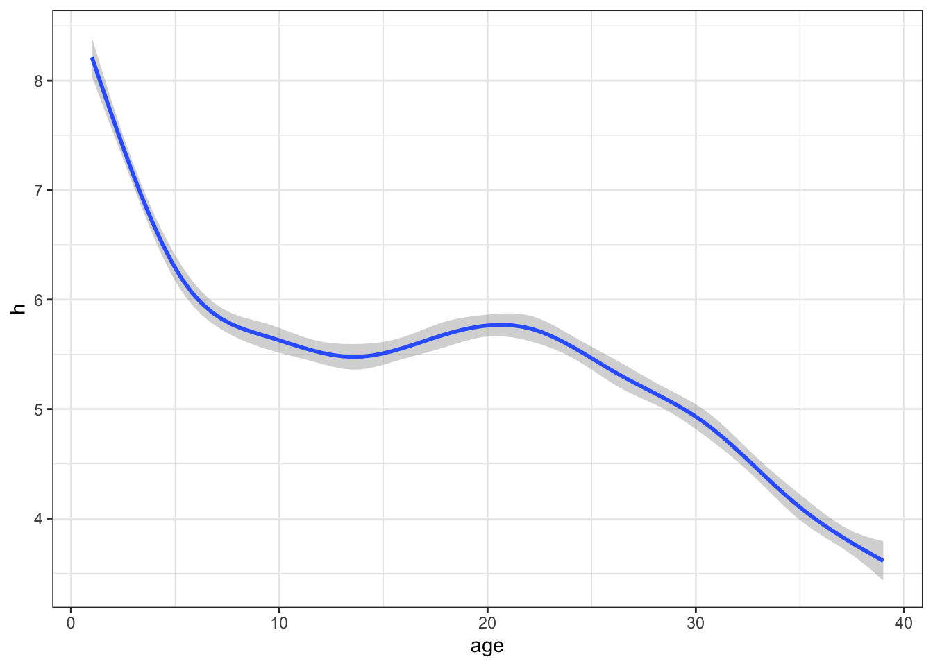

# compute asset 
ggplot(simdata,aes(x=age,y=lb)) + geom_smooth()

## `geom_smooth()` using method = 'gam' and formula 'y ~ s(x, bs = "cs")'

## Warning: Removed 2072 rows containing non-finite values (stat_smooth).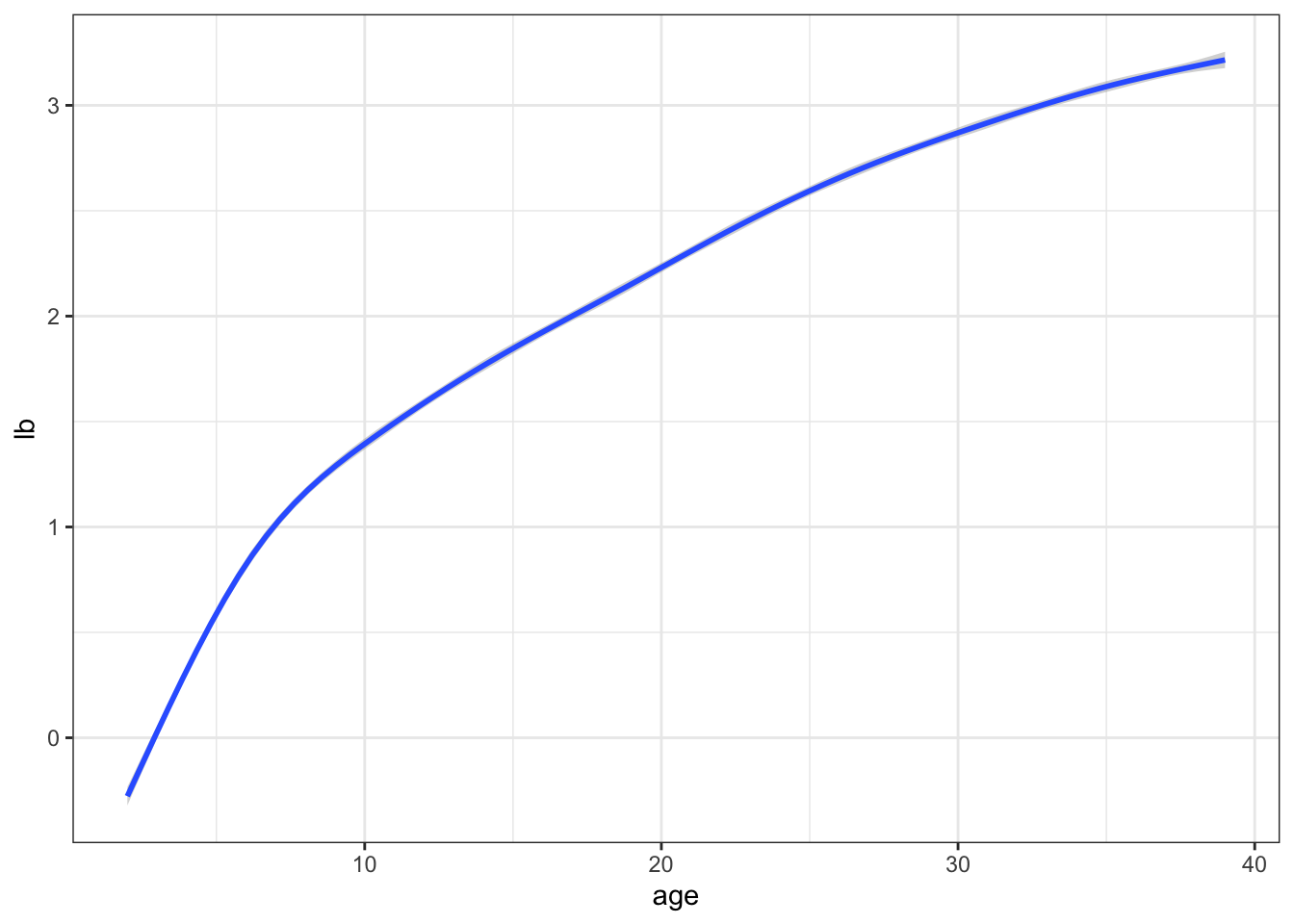

simdata[,hist(h)]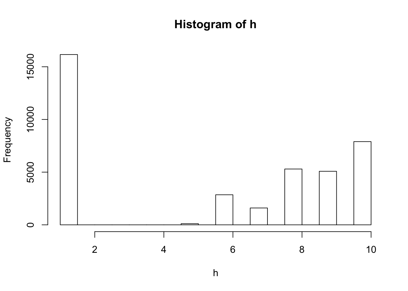

## $breaks
##  [1]  1.0  1.5  2.0  2.5  3.0  3.5  4.0  4.5  5.0  5.5  6.0  6.5  7.0  7.5  8.0
## [16]  8.5  9.0  9.5 10.0
## 
## $counts
##  [1] 16161     0     0     0     0     0     0   111     0  2853     0  1599
## [13]     0  5297     0  5082     0  7897
## 
## $density
##  [1] 0.828769231 0.000000000 0.000000000 0.000000000 0.000000000 0.000000000
##  [7] 0.000000000 0.005692308 0.000000000 0.146307692 0.000000000 0.082000000
## [13] 0.000000000 0.271641026 0.000000000 0.260615385 0.000000000 0.404974359
## 
## $mids
##  [1] 1.25 1.75 2.25 2.75 3.25 3.75 4.25 4.75 5.25 5.75 6.25 6.75 7.25 7.75 8.25
## [16] 8.75 9.25 9.75
## 
## $xname
## [1] "h"
## 
## $equidist
## [1] TRUE
## 
## attr(,"class")
## [1] "histogram"